This material concerns Dr. Randell Mills's alternative
theory of Quantum Mechanics, known as "the Grand Unified Theory of Classical Physics", or
GUT_CP. I am a firm believer that Dr Randell Mills of Blacklight Power has made some major
discoveries in Physics, such as his discovery that the Hydrogen atom can collapse to energy
levels below that which is conventionally considered to be the ground state of atomic hydrogen.
On studying GUT_CP I have found that the mathematics can be excessively complex, and also that in
parts of the theory there are what appear to me to be inconsistencies.
The material here is an Alternative Presentation of some of the concepts in GUT_CP.
Suppose we have a structure in a 3D (or 2D) coordinate system. A RESIDUE ROTATION of the structure is defined as
the structure formed as we rotate the structure about an axis (or point) through a large angle by means of a series of successive small angular steps,
and we deposit an image of the structure at each successive small angular step. We shall call the angle value used in small angular step the PITCH of the Residue Rotation.
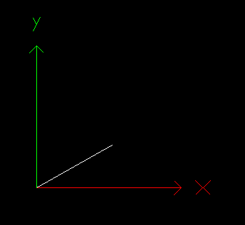
To demonstrate, here we have an XY coordinate system, and a line segment in the first quadrant:
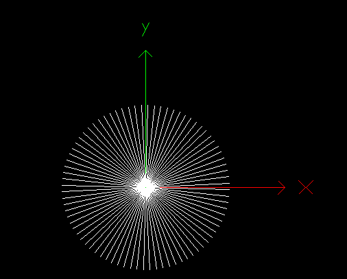
When we RESIDUE ROTATE this line segment through 2*PI radians about the origin, we get this image, the "SPOKES OF WHEEL":
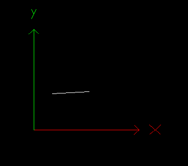
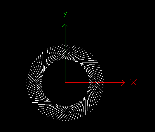
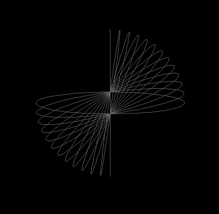
Similarly, if we start out with a Line Segment away from the origin:
We perform RESIDUE ROTATION about the origin, and we get the "TYRE TREADS":
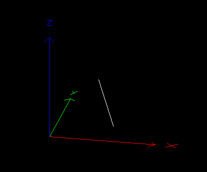
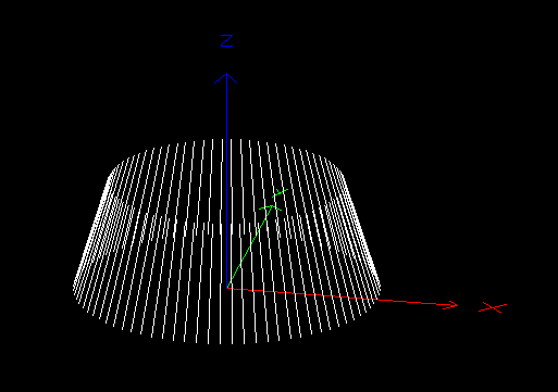
In 3 dimensions, next we start out with a Line Segment with one endpoint in XY plane, the other endpoint above it in Z-value and directly towards the Z-axis:
We Residue Rotate this Line Segment about the Z-axis, and we get the "LAMPSHADE":
The pdf file explains two ways of forming the Orbitsphere using Residue Rotations. View pdf file
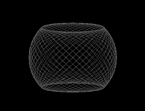
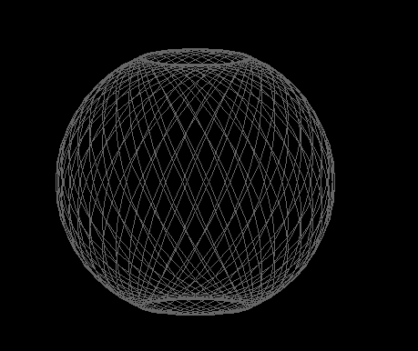
Start out with a Great Circle of current in the XY plane. Tilt this Great Circle through an angle theta_tilt, about the Y-axis. Then Residue Rotate about the Z-axis, through 2PI.
The result is what I call the String Barrel, a shape familiar to those who have looked at the early chapters of GUT_CP:
We can chooses different values of theta_tilt. Above was PI/4.
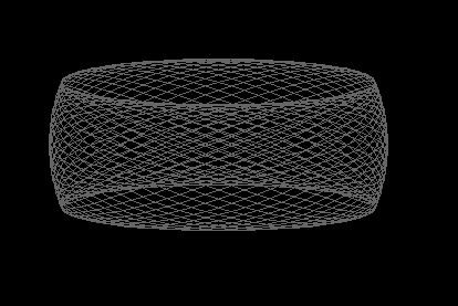
Here are the String Barrels for different theta_tilt values:
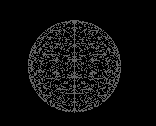
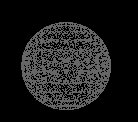
We superpose several String Barrels of different theta_tilt, and the result is the Orbitsphere:
The PITCH of the Residue Rotation, and the value delta(theta_tilt) were adjusted to be equal in the above image.
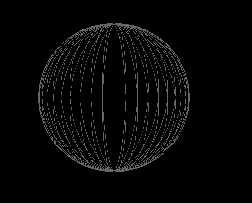
Start out with a Great Circle in the XY plane. Residue Rotate through PI/2 about the Y-axis. The result is the
"FAN OF GREAT CIRCLES":
Then Residue Rotate the Fan of Great Circles about the Z-axis through 2PI:
Again, the respective pitches were adjusted to be equal.
4) The Normalization Factor
In the above construction of the Orbitsphere, it was assumed that the current in each Great Circle is constant.
When one asks the question, "What is the Charge Density on the Orbitsphere?" one notices that though the Charge Density may
be symmetric about the Z-axis, it is not constant for points on the Orbitsphere of differing Z-values. In fact around the Equator
there appears to be a Charge Surplus, and similarly around the Poles.
To seek a Uniform Charge Density on the Orbitsphere, one can try multiplying the charge on Great Circles of particular tilt angles
by a constant Normalization Factor, which I call G.
This pdf file describes the calculation of G, and also demonstrates
that if we use this G-value we do indeed get the desired Uniform Charge Density.
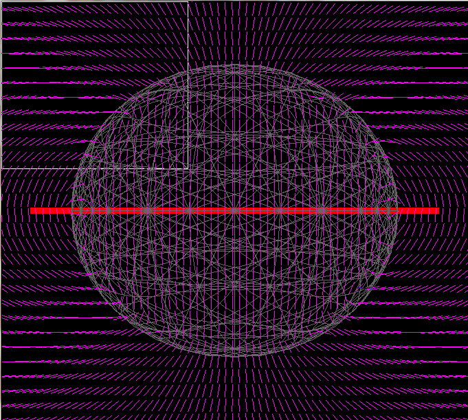
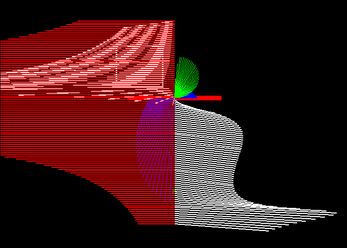
5) Magnetic Field due to the Orbitsphere current pattern - Computer Simulation
The next image shows the output from a C++/OpenGL program I have written which uses the Biot-Savart Law to
calculate the Magnetic Field inside and in the region just outside the Orbitsphere. In GUT_CP, Dr Mills asserts that the Magnetic Field
is uniform inside the Orbitsphere and like a dipole outside the Orbitsphere. My opinion is that this statement is approximately but
not exactly correct. Ignore the white box and the red bar - they are just there as an aid to the Programmer.
6) Ellipsoidal Analogue of the Orbitsphere - Two Theorems
Suppose we have an Ellipsoid which is formed by stretching a sphere in one direction so
that the direction of stretching becomes the major axis of the Ellipsoid. Then a cross section of the Ellipsoid through the Major Axis
contains the two foci of the Ellipsoid F1 and F2, which according to GUT_CP are the locations of the two nuclei in Dr. Mills's model of a diatomic molecule.
The next pdf file demonstrates the following theorem. If we intersect a plane with the Ellipsoid such that the plane includes the focus F1, then the
intersection of the plane with the Ellipsoid is an ellipse with one of its two foci coincident with F1.
View pdf file 1
The next pdf is of two sections. The first section is one page which illustrates a simple model of a diatomic molecule consisting
of two positive charges located along the X-axis, and a circular ring of negative charge in the mid-plane between them.
The next section demonstrates another Theorem related to the Ellipsoidal analogue of the Orbitsphere.
We have a positively charged nucleus at the origin, and we have a Filamentary Ellipse of negative charge orbiting around the nucleus according
to Coulombs Law. There is no self-interaction in the Filamentary Ellipse. It is proven that the net force on the nucleus from this Filamentary
Ellipse is zero. View pdf file 2
These two Theorems taken together imply that one can indeed have an Ellipsoidal analogue of the Orbitsphere, in which the nucleus is at the focus F1
and the electron charge moves about the nucleus in a Ellipsoidal pattern made of filamentary ellipses.
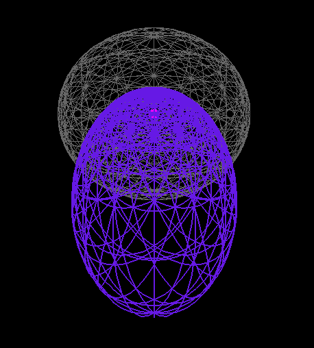
The next image shows the Ellipsoidal analogue of the Orbitsphere drawn over a spherical Orbitsphere. There is a pink ball - the nucleus - just
visible at the upper focus of the Ellipsoid.
7) Electric Field along Ellipsoid Major Axis - Computer Simulation
Since the Ellipsoidal analogue of the Orbitsphere is to be used to model the Diatomic Molecule, the next step is to find out what the Electric Field
is at points along the major axis of the Ellipsoid, with particular interest in the value of the Electric Field at the Secondary Focus of the Ellipsoid.
Denoting the origin as the Primary Focus and setting the Z-axis along the Ellipsoid's Major Axis (up=+Z in above image), it is then necessary to calculate the Z-component of
the Electric Field by applying Coulomb's Law to individual pieces of each Filamentary Ellipse and performing a summation.
What about the Normalization Factor, G, for each Filamentary Ellipse? We assume it is the same as it would be for a similarly-oriented Orbitsphere.
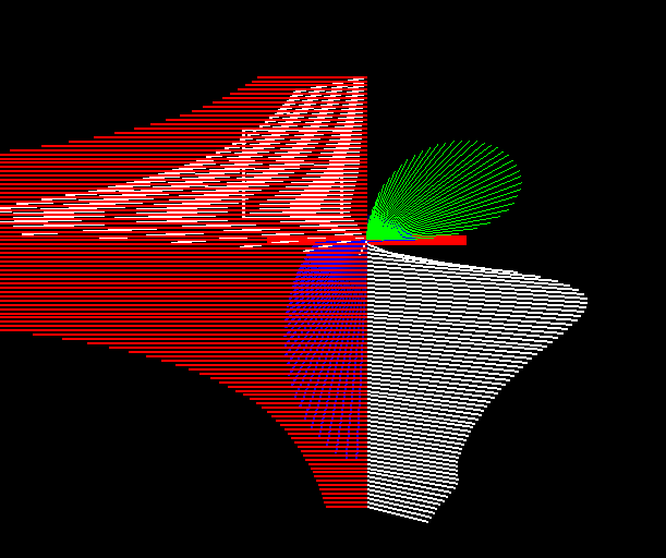
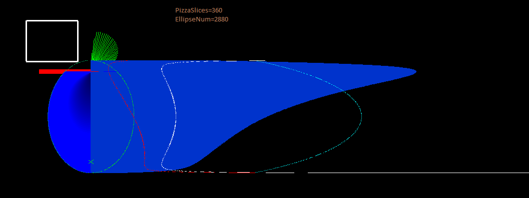
The result:
The Blue lines are a Fan of Filamentary Ellipses - it is only necessary to have one Fan since we are only interested in the
Z-component of the field not the X and Y components.
The Green lines are proportional in length to the Normalization Factor for Filamentary Ellipses oriented in those directions. That is, Green Line and projection of
corresponding Filamentary Ellipse are collinear in the diagram.
The White line gives a measure of the magnitude of the Z-component of the field due to the Filamentary Ellipses of negative charge.
The Red line is proportional in length to the Coulomb force from the nucleus at the primary focus of the Ellipsoid. Magnitude of nuclear
charge = Magnitude of negative charge in Filamentary Ellipses.
What we want in order to be able to model a Diatomic Molecule is for the red and white lines to be of equal length at the Secondary Focus,
indicating that, when we introduce a second Nucleus at the Secondary Focus, the repulsion from the first nucleus is balanced by an equal
and opposite force from the Ellipsoid pattern of negative charge. In the above diagram, this does not happen, however, what one can do
is tweak the Normalization Factor until we get Force Balance.
The next image is displayed as above but for the tweaked Normalization Factor, which is the previous Normalization Factor
multiplied by a weighting function consisting of an off-centre arch of sine curve.
At the Secondary Focus, there is Force Balance to a good degree of accuracy.
9) the Topological Postulate
Thus, in this model we can introduce a Secondary Nucleus at the Secondary Focus of the Ellipsoid. The Second Nucleus is repelled
by the First Nucleus, but is also pulled towards the First Nucleus by the Negatively Charged Ellipsoid of Filamentary Ellipses
orbiting the First Nucleus. The Secondary Nucleus also brings with it an Ellipsoid of negative charge which exerts zero net force
on it, and which superposes with the Ellipsoid from the First Nucleus.
The question one can ask about this model is: When we introduce the Second Nucleus, why does it not disturb the charge pattern of the
Ellipsoid due to the First Nucleus? I propose that the Electron Ellipsoid feels NO FORCE from the Secondary Nucleus due to the following
postulate:
When an electron forms an Orbitsphere or Ellipsoid, it experiences a Coulomb force from only ONE POINT, or ONE TINY LOCALIZED REGION of the
volume enclosed by the concave surface of the electron charge pattern.
I call it the Topological Postulate because there is a topological difference between those points within and those points without the
concave surface of the Orbitsphere / Ellipsoid / Other Closed Shape.
Thus I have presented an Orbitsphere-based model of the Diatomic Molecule, a modified version of the model presented in GUT_CP chapter 11,
in which force balance is achieved.
The model in GUT_CP chapter 11 has the following drawbacks:
1- it assumes that the electron charge moves on an Ellipsoidal equipotential, however, if one uses Coulomb's Law to calculate the field pattern
due to two positive point charges, one does not get a pattern with Ellipsoidal equipotentials.
2- Even if the electron charge were to somehow reside on an Ellipsoid of constant potential, then this Ellipsoid is effectively a Faraday Cage
enclosing the nuclei at the foci, and then the field within the Faraday Cage from the negatively charged electrons is zero, and so there is no extra
negative charge to stop the nuclei pushing apart.
3- GUT_CP chapter 11 describes the Filamentary Ellipses as being centred on the midpoint between the two nuclei and does not explain
why they should have these orientations and motions.
The Alternative Model has none of these drawbacks - it merely requires us to accept the Topological Postulate and apply Coulomb's Law.
BLUE CURVE: The length of each horizontal blue line from the major axis to the right is proportional to the total charge on the Ellipsoid at that Z-value.
CYAN CURVE (not ellipsoid outline): Measured from major axis, gives measure of d(surface area)/dZ.
RED CURVE: Measured from major axis, proportional to Surface Charge Density dQ/d(surface area) for ONE ELECTRON ELLIPSOID.
WHITE CURVE: Measured from major axis, proportional to Surface Charge Density dQ/d(surface area) for TWO SUPERPOSED ELECTRON ELLIPSOIDS.
The formula U = k_coulomb * Q1 * Q2 * 1/r can be used to find the energy required to assemble the Diatomic Molecule.
We start out with nucleus N1 at the origin, then we find the energy required to bring nucleus N2 to its respective point, then we subtract the energy released by bringing
electron 1 from infinity to its Ellipsoid pattern minus that which goes into kinetic energy. We do similarly for the second electron.
Then comes the tricky part: We must calculate the energy required to bring the second electron from infinity to its Ellipsoidal pattern working against
the field from the first electron's Ellipsoidal pattern. We can use the above formula applied to elementary pieces of filamentary ellipses, but considerable computational resources are
required.
 Ben Jones, MPhys., MSc.